 Generalized phase method Generalized phase method
|
 Trace of the Diagram Trace of the Diagram
|
 Scheme search by the generalized phase method Scheme search by the generalized phase method
|
 Footer Footer |
Sequential Logic Schema Search :
2. - RESEARCH OF THE SCHEMES IN SEQUENTIAL LOGIC
This chapter presents a certain amount of information which, while very important in automatism and somewhat beyond the scope of this lesson, is not essential to understanding the digital electronic systems that will follow.
2. 1. - SEARCH FOR A DIAGRAM BY PAR BY THE METHOD OF PHASES (bottom of page)
Suppose that, to control the ignition of a lamp L, there are two push buttons, one called «m» or «on» and the other «a» or «off».
Figure 5 shows the operating table of the assembly.
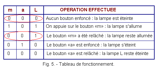
We can see by examining Figure 5 that for two identical combinations of input variables «a» and «m» there are two different logical states for L (combinations circled in red).
This is new. We can not solve the problem by the traditional combinatorial method. Indeed, the Karnaugh table only admits a value 1 or 0 per box or combination of input variables.
This is why it is necessary to introduce a secondary variable called memory which allows to keep the memory of the previous events and to establish a chronology. In electrical technology, this memory is materialized by an X relay which is an output variable and its contact x which is a new input variable.
The previous state of the output (given the delay introduced) is thus taken into account as an additional input variable called secondary variable. It is called internal variable, in electronics.
For convenience, we will take X = L, which is not mandatory ; indeed, one could also imagine X = f (L).
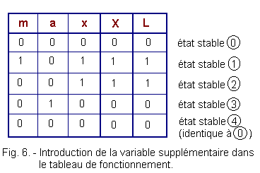
We can rewrite the operating table as shown in Figure 6.
In Theory 2, we have seen the use of Karnaugh's tables in which the input variables were independent of the outputs. Now, this is no longer the case because L = X = x and a variation of L causes a variation of x. We have to do here, sequentially, circuits looped on themselves for which we can not use the method of Karnaugh. From the new operating table where each combination of the inputs determines a stable state of the outputs, we can represent by means of a graph called the chronogram the evolution of m, a, x, X and L as a function of time (Figure 7). The timing diagram of Figure 7 takes into account the delay in the rise of the relay X, indeed, there is a time
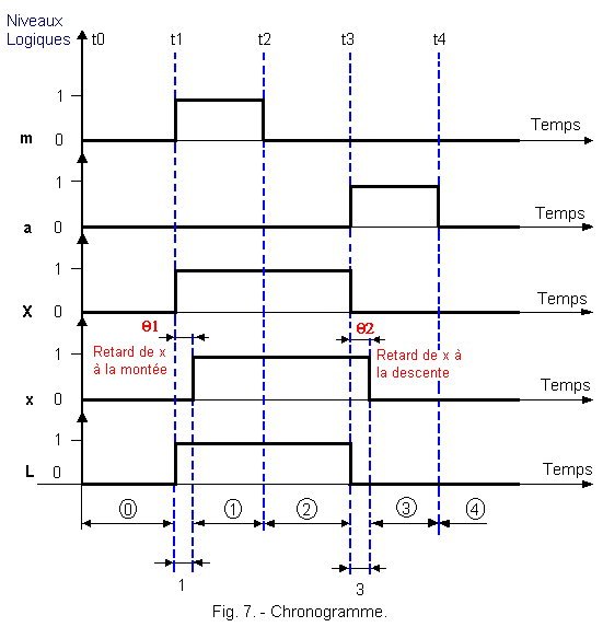
We will call, transitory, the times q1 and q2 of sticking and taking off of the contac x of the relay X.
We see that L will be lit during the phases : transient 1, OR steady state ![]() ,
OR stable state
,
OR stable state ![]() .
.
We can therefore write by looking at the chronogram for 1, ![]() ,
,
![]() will L = X be equal to :
will L = X be equal to :
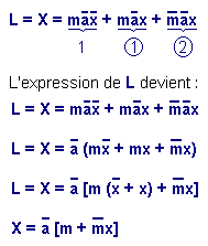
Now, as we saw in a previous theory
: a + ![]() b
= a + b so X =
b
= a + b so X = ![]() (m + x). (Back next)
(m + x). (Back next)
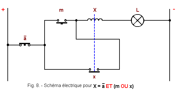
The diagram of Figure 8 materializes the equation found.
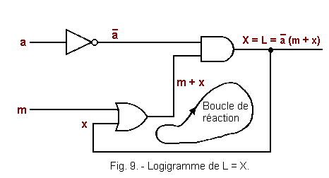
The logic diagram is represented by Figure 9.
Looking at Figure 9, we can notice that the delay between X and x does not appear ; however, there is a delay due to the transit time through the OR gate and the AND gate conditioning the reaction loop Figure 9.
These notions of transit time are specified in the theory 5 as well as in the technology 4 entitled "Summary Digital and Fundamental Technology".
Knowing that according to DE MORGAN's theorem it is possible to replace an AND by a NOR with the complemented inputs and that on the other hand an OR can be replaced by a NOR followed by an inverter, the diagram becomes that of Figure 10.
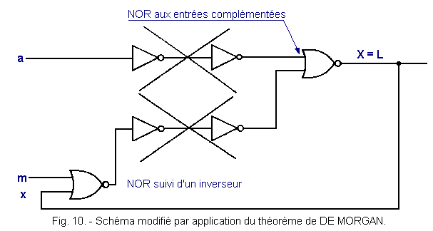
The simplified diagram is then that of Figure 11.
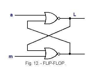
The circuit obtained is a flip-flop Bistable on-off.
.gif)
A much more widespread representation of this same circuit is given in Figure 12. This montage is still called FLIP-FLOP : We will talk about it quite a bit later.
![]() 2. 2. - GENERAL PHASES METHOD
2. 2. - GENERAL PHASES METHOD
A method that we will not demonstrate here because it goes well beyond the scope of this lesson makes it possible to replace algebraic simplification with Karnaugh's tables.
This extended phase method can be applied to all sequential devices.
Phase is the time during which a transient or stable state occurs.
2. 2. 1. - DIAGRAM OF PHASES
The phase diagram is represented by a grid (Figure 13).
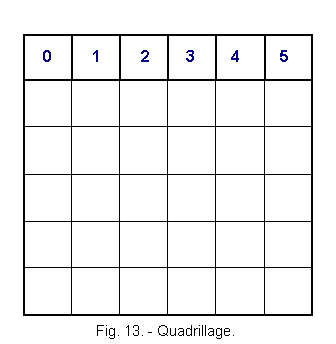
a) At the top of each column, the number of the phase is indicated. Whatever the duration of the phases (a few nanoseconds or a few seconds) the columns will be identical.
b) Indicate, Figure 14, in front of each line, successively in the order of their implementation :
![]() The input variables in lowercase.
The input variables in lowercase.
![]() The excitation organism (s) identified by capital letters.
The excitation organism (s) identified by capital letters.
![]() The secondary transfer variable or variables in the order of their use represented by lowercase letters.
The secondary transfer variable or variables in the order of their use represented by lowercase letters.
![]() The output (s) in capital letters.
The output (s) in capital letters.
For each input variable and each secondary transfer variable, we define a weighting p which is a number such that for the first input variable p = 21 - 1 = 1, for the second variable p = 22 - 1 = 2..., for the nième variable p = 2n - 1.
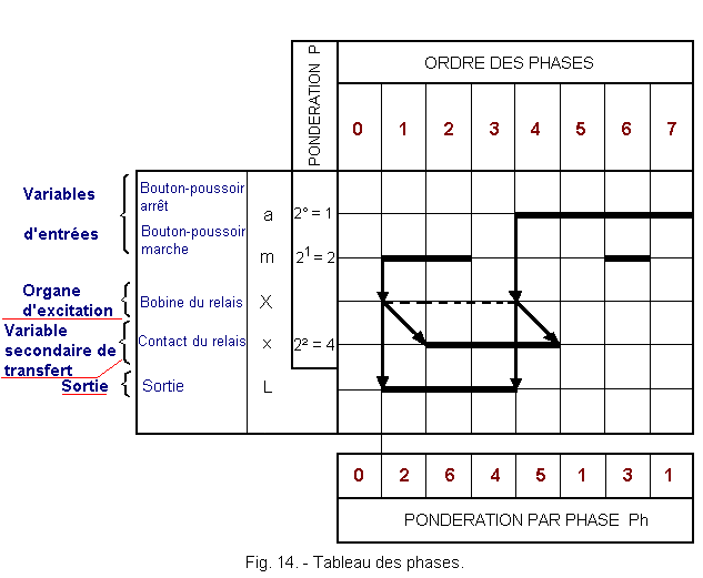
In the example already solved previously, the phase table is shown in Figure 14.
![]() 2. 2. 2. - TRACED
DIAGRAM
2. 2. 2. - TRACED
DIAGRAM
Let's look at the table in Figure 14.
Phase 0 conventionally represents the state of rest of the system.
The bold lines drawn on the horizontal lines of the table corresponding to the variables, represent these variables or contacts in state 1 during each phase.
The horizontal discontinuous bold lines represent the state 1 of the excitations in each phase.
Whenever the modification of the state of an input variable (including secondary variables) results in a change of state of an output (including excitations) this is indicated by a vertical arrow (in bold).
However, the dependencies between excitations and secondary transfer variables will be marked by oblique arrows to take into account the appreciable delay (time q = of transfer) introduced by the back-coupling.
The Ph phase weighting shown in the table is the sum of the p-weightings of each state variable 1 (inputs and transfers), performed vertically within a given phase.
Diagram rules :
![]() Only one variable must change at each phase.
Only one variable must change at each phase.
![]() The secondary variables are always delayed by one phase with respect to the excitation state.
The secondary variables are always delayed by one phase with respect to the excitation state.
![]() An identical weighting in two phases but producing different states of the excitations or the outputs necessarily introduces a new secondary variable : one must add an additional excitation and its transfer.
An identical weighting in two phases but producing different states of the excitations or the outputs necessarily introduces a new secondary variable : one must add an additional excitation and its transfer.
We will now see in more detail how we came to developing the table in Figure 14.
![]() 2. 2. 3. - RESEARCH
OF THE SCHEME OF PARAGRAPH 2. 1. BY THE METHOD OF GENERALIZED PHASES
2. 2. 3. - RESEARCH
OF THE SCHEME OF PARAGRAPH 2. 1. BY THE METHOD OF GENERALIZED PHASES
a) Analysis of information
The very important starting point of this method is the analysis of the information available and the elaboration of a functioning table.
This one must show in a precise way the various possible cases of figures for the state of the entries and the state of the outputs for each one of these combinations.
Figure 15 gives the operating table for the case we are interested in (Figure 8).
.gif)
b) Construction of the diagram.
From the previous operating table, let's start to draw up the system phase table ; this table represented in Figure 16 comprises three horizontal lines since there are two input variables a and m and an output L.
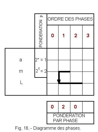
The table can be broken down vertically as follows :
Phase 0 :
Rest position a = 0, m = 0, L = 0
No organ is actuated, there is no need to draw a line in bold.
The Ph weighting of this phase is 0.
Phase 1 :
a = 0, m = 1, L = 1
Pressing m lights the lamp. A bold line is drawn for m and L. The Ph weighting is 2. The vertical arrow indicates that m = 1 leads to L = 1.
Phase 2 :
a = 0, m = 0, L = 1
The bold line of phase 1 is extended to L. The Ph weighting of this phase is 0.
WARNING :
For the phases 0 and 2, the weighting is 0, but the input variables are in both cases at 0. As we pointed out previously, it is thus necessary to introduce a secondary variable to differentiate these two cases.
A complementary relay X and its secondary transfer variable x allows this discrimination by changing the weighting of phase 2.
Figure 17 shows the new phase table obtained with these new data.
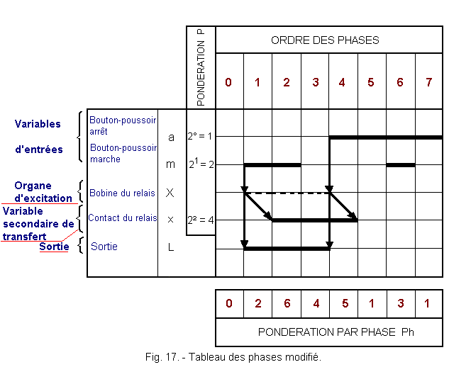
Phase 1 :
a = 0, m = 1, L = 1
The action of m causes the excitation of X (vertical arrow oriented from m to X).
The action of m also causes the ignition of L hence the extension of the arrow vertically towards L.
The x transfer contact controlled by X is one phase late with respect to the excitation (an oblique arrow pointing from X to x is drawn).
If we release m during phase 1, let L be extinguished. To overcome this hazard, x is not yet 1, it is necessary to extend the action of m during the next phase to ensure that the pulse on m has been stored.
This will always be done when a variable will excite a new relay.
The weighting of phase 1 will be 21 = 2.
Phase 2 :
a = 0, m = 1, L = 1
A single variable changes state with respect to the phase, in fact, only x goes to 1 whereas m, as we decided in phase 1 was kept at 1, X remaining stuck.
It is necessary to prolong the bold line of m, the dotted line of X, the bold line of L. The weighting Ph passes to 6.
Phase 3 :
a = 0, m = 0, L = 1
Release m (the bold line stops), the excitation X is memorized by x (the dotted lines are extended on X and the bold lines on x and L). Between phases 2 and 3, only one variable changes state : m is released.
The Ph weighting of this phase is 4.
Phase 4 :
a = 1, m = 0, L = 0
Pressing "a" causes X to go to 0 and L also. We draw a vertical line arrowed towards X and towards L.
x will follow X with a delay of one phase.
We draw an oblique line from X of x.
We realize that if we release "a" during phase 4 while "x" has not changed state, a malfunction may occur ; L reigniting because the action on "a" was not memorized by "x", secondary input variable.
It is therefore necessary to extend the influence of "a" in the next phase.
The Ph weighting of this phase is 5.
Phase 5 :
a = 1, m = 0, L = 0
The action on "a" is prolonged, we draw the bold line. There is no more excitement of transfer. The Ph weighting of this phase is 1.
Phase 6 :
a = 1, m = 1, L = 0
This phase makes it possible to highlight the case where the action on "a" is prolonged and that "m" is pressed.
We draw two solid lines. Priority is given to the stop, the action on "m" has no effect so there is no need to draw other features.
Phase 7 :
To return to phase 0 ("a" and "m" released), it is necessary to go through phase 7 so that only one variable switches. We prolong the action of "a".
Phases 5 and 7 have the same weighting and are identical, the action on "a" causing no change.
By maintaining "m" and releasing "a" we would have fallen back to phase 1.
All cases have been considered, the diagram is complete.
c) Deduction of the equation of the output (lamp L).
We have seen in Chapter 2. 1. that it is possible to draw the equation directly from the diagram. But in the case where several secondary variables are needed (and the number is unknown when reading the problem statement) this is practically impossible and the hazards are more difficult to detect.
Let's use Karnaugh's painting.
The table is composed of 2n boxes (n representing the total number of primary and secondary variables).
In order to avoid operational hazards in electronics and electricity, it is mandatory to perform overlapping groupings.
![]() Let's number the cells of Karnaugh's table in decimal (Figure 18) according to the binary weight of the entries for example for the box :
Let's number the cells of Karnaugh's table in decimal (Figure 18) according to the binary weight of the entries for example for the box :

![]() Define the value 1 in the boxes whose decimal number corresponds to the Ph weighting per phase for which X = 1.
Define the value 1 in the boxes whose decimal number corresponds to the Ph weighting per phase for which X = 1.
Karnaugh's chart is set for each excitement, here only one : X, so one table. The table obtained is that of Figure 18.
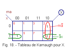
From the table, we draw the following equation :
X = m![]() +
+ ![]() x
x
X = ![]() (m
+ x)
(m
+ x)
The equation found is very similar to that obtained in Chapter 2. 1.
Just do and draw the flow chart that you can find Figure 9.
 Click here for the next lesson or in the summary provided for this purpose. Click here for the next lesson or in the summary provided for this purpose. |
|
 Previous Page Previous Page |
 Next Page Next Page |
Nombre de pages vues, à partir de cette date : le 27 Décembre 2019
Envoyez un courrier électronique à Administrateur Web Société pour toute question ou remarque concernant ce site Web.
Version du site : 10. 4. 12 - Site optimisation 1280 x 1024 pixels - Faculté de Nanterre - Dernière modification : 02 Septembre 2016.
Ce site Web a été Créé le, 14 Mars 1999 et ayant Rénové, en Septembre 2016.
