 Footer Footer |
Matrix Method of Huffman and Fusion Polygon :
2. 3. - HUFFMAN MATRIX METHOD
We know that Karnaugh's chart does not directly solve a sequential problem. Indeed, for each combination of the input variables, there can only be one value for the output, that is to say one value per elementary box of the array.
It is therefore necessary to look for a representation that allows the introduction of one or more secondary variables as seen previously.
2. 3. 1. SEQUENCE
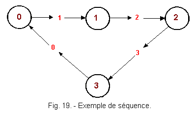
A sequence is a looped succession of stable states separated by transient states.
Figure 19 shows an example of a sequence.
2. 3. 2. - RESOLUTION OF A PROBLEM BY THE MATRIX METHOD
To illustrate this method, let's take the same example again.
a) Analysis
There are two input variables «m» and «a».
These two variables make it possible to obtain 22 = 4 combinations.
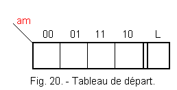
As a starting point, we use a table with four columns corresponding to the combinations of entries that are arranged according to the reflected binary code. In a fifth column, enter the binary value of the output state. The table is shown in Figure 20.
Let us take again the operation of the assembly and define the number of stable states :
![]() Initial state
a = 0, m = 0 with L = 0
Initial state
a = 0, m = 0 with L = 0
![]() Action on m
a = 0, m = 1 where L = 1
Action on m
a = 0, m = 1 where L = 1
![]() m is released
a = 0, m = 0 and L always at 1
m is released
a = 0, m = 0 and L always at 1
![]() Action on a
a = 1, m = 0 and L = 0
Action on a
a = 1, m = 0 and L = 0
![]() Simultaneous action on a
and m
a = 1, m = 1 we chose to privilege the stop :
Simultaneous action on a
and m
a = 1, m = 1 we chose to privilege the stop :
b) Construction of the primitive matrix of states.
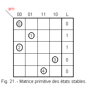
A primitive matrix of states is a table of the model of Figure 20 in which there is a stable state line as shown in Figure 21.
Each stable state is positioned in the box for which the variables «m» and «a» are at the values having caused this stable state.
Example :
For a = 0, m = 0
stable state ![]() ,
L = 0
,
L = 0
a = 0, m = 1
stable state ![]() ,
L = 1
,
L = 1
a
= 0, m = 0
stable state ![]() ,
L = 1
,
L = 1
a
= 1, m = 0
stable state ![]() ,
L = 0
,
L = 0
a
= 1, m = 1
stable state ![]() ,
L = 0
,
L = 0
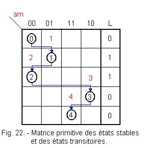
It is now necessary to position the transient states.
The transient states are located at the intersection of the line on which the initial stable state appears and the column in which the next steady state appears.
Figure 22 shows these transient states.
We know that it is impossible for two variables to switch simultaneously. To materialize this on the primitive matrix, it is necessary to hatch to eliminate them, all the boxes for which on the same line two variables change with respect to the combination of the variables which caused the stable state included in this line.
We thus obtain the table of figure 23.
In our example : for steady state ![]() a = 0, m = 0, you have to hatch the box where a = 1, m = 1
a = 0, m = 0, you have to hatch the box where a = 1, m = 1
for steady state ![]() a = 0, m = 1, you have to hatch the box where a = 1, m = 0
a = 0, m = 1, you have to hatch the box where a = 1, m = 0
for steady state ![]() a = 0, m = 0, you have to hatch the box where
a = 1, m = 1
a = 0, m = 0, you have to hatch the box where
a = 1, m = 1
for steady state ![]() a = 1, m = 0, you have to hatch the box where a = 0, m = 1
a = 1, m = 0, you have to hatch the box where a = 0, m = 1
for steady state ![]() a = 1, m = 1,
you have to hatch the box where a = 0, m = 0
a = 1, m = 1,
you have to hatch the box where a = 0, m = 0
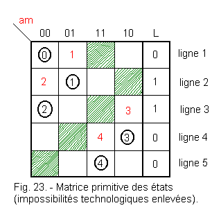
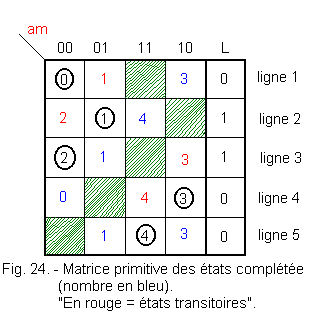
It is now necessary to examine the remaining boxes.
Line 1 :
Box 10 (a = 1, m = 0)
If we press "a" while L is off, we move to a steady-state situation ![]() (a = 1, m = 0, L = 0), so we write 3 in the box which shows that we go through the transient state 3.
(a = 1, m = 0, L = 0), so we write 3 in the box which shows that we go through the transient state 3.
Line 2 :
Box 11 (a = 1, m = 1)
If we press "a" while "m" has not been released, we go to the extinction of the lamp so to the steady state ![]() (a = 1, m = 1, L = 0). We write 4
in the box.
(a = 1, m = 1, L = 0). We write 4
in the box.
Line 3 :
Box 01 (a = 0, m = 1)
If we press «on» while the lamp is already on, this has no effect and we go to the steady state ![]() (a = 0, m = 1, L = 1), we write 1 in the box.
(a = 0, m = 1, L = 1), we write 1 in the box.
Line 4 :
Box 00 (a = 0, m = 0)
We release "a" and the lamp remains off, so we go to steady state ![]() (a = 0, m = 0, L = 0), we write 0 in the box.
(a = 0, m = 0, L = 0), we write 0 in the box.
Line 5 :
1) Box 01 (a = 0, m = 1)
We release "a" while "a" and «m» were activated and L was extinguished. The lamp comes back because we return to the stable state ![]() (a = 0, m = 1, L = 1), so we write 1 in the box.
(a = 0, m = 1, L = 1), so we write 1 in the box.
2) Box 10 (a = 1, m = 0)
We release the start button while L is off, we return to the stable state ![]() (a = 1, m = 0, L = 0), so we write 3 in the box.
(a = 1, m = 0, L = 0), so we write 3 in the box.
The primitive matrix completed in Figure 24 is thus obtained.
c) Finding the contracted matrix
It is desirable to reduce the original matrix of states to a contracted matrix in order to reduce the number of additional lines, which introduce new excitations and new complementary variables or transfers.
Contraction or merger rules :
![]() It is possible to contract the primitive matrix of states by superimposing two lines if they present vertically the same states.
It is possible to contract the primitive matrix of states by superimposing two lines if they present vertically the same states.
![]() Two lines can be merged into one when there is a steady state or a transient of the same number in the same column or a stable or transient state with a hatched box in the same column, because the hatched box indicates that, for technological reasons, this case can not occur and is therefore indifferent.
Two lines can be merged into one when there is a steady state or a transient of the same number in the same column or a stable or transient state with a hatched box in the same column, because the hatched box indicates that, for technological reasons, this case can not occur and is therefore indifferent.
![]() Output states do not intervene in the possible overlays.
Output states do not intervene in the possible overlays.
Study of the possibilities for line 1 :
Let's compare line 1 with line 2 : they are not superimposable because for a = 0 and m = 0, we have the state ![]() on the first line and 2 on the second.
on the first line and 2 on the second.
Let's compare line 1 with line 3 : they are not superimposable because we have ![]() on the first line and 2 on the third for a = 0 and m = 0.
on the first line and 2 on the third for a = 0 and m = 0.
Let's compare line 1 with line 4 : these two lines are superimposable because we have ![]() corresponds to 0, to 1 corresponds an impossibility, to an impossibility corresponds 4, to 3 corresponds
corresponds to 0, to 1 corresponds an impossibility, to an impossibility corresponds 4, to 3 corresponds ![]() .
.
Let's compare line 1 with line 5 : these two lines are superimposable.
For line 2, the possible combinations are :
Lines 2 and 3 stackable.
Lines 2 and 4 are not stackable.
Line 2 and 5 stackable.
For line 3, the possible combinations are :
Lines 3 and 4 non-stackable
Lines 3 and 5 stackable
For line 4, the possible combinations are :
Lines 4 and 5 stackable
d) Fusion polygon
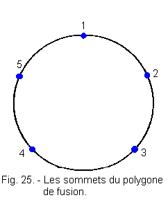
Let's spread on a circle by counting in a clockwise direction the five points representing the five lines of the primitive matrix of states : we get Figure 25.
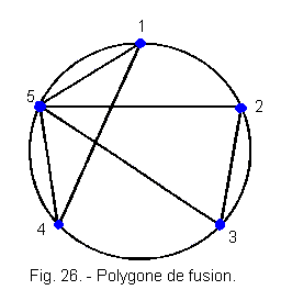
Connect together all the stackable lines as shown in Figure 26.
e) Interpretation of the fusion polygon
We get two triangles of vertices 1-5-4 and vertices 2-5-3.
Rule :
For example, we can merge 2-3-5 ... n vertices connected to each other, but each vertex must appear in only one group so that in our case we can make the groupings :
1-4-5 and 2-3 or 2-3-5 and 1-4
We will prefer 1-4-5 and 2-3 because inside each group the state of the outputs is identical.
This will later facilitate the groupings in the final table of Karnaugh, but it is not obligatory and especially not always possible.
f) Contrasted matrix or fusion table.
Let's superimpose lines 1-4-5 shown in Figure 27.
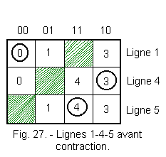
Figure 28 shows lines 1-4-5 after contraction.
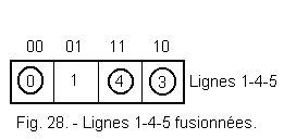
Figure 28 shows that stable states outweigh transitions on fusion.
Figure 29 shows lines 2-3 of the primitive matrix before merging.
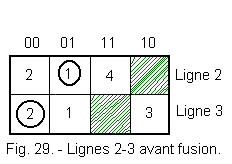
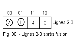
Figure 30 shows lines 2-3 after merging.
We can reconstruct a so-called contracted matrix using lines 1-4-5 and 2-3. Figure 31 shows this contracted matrix.
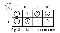
We see in Figure 31 that the contracted matrix comprises two lines, which means that the complementary variables or transfers are only one number that we call x.
For a matrix of 21 = 2 lines, we have 1 complementary variable, for 22 = 4 lines, we have 2 complementary variables and for 2n lines we have n variables.
If the matrix includes 20 = 1 line, the system under review can be summarized as a combinatorial system (no additional variables).
g) Establishment of Karnaugh's chart reducing the problem to a combinatorial problem.
Let's establish Karnaugh's array of output by plotting the output binary values for the stable states considered in the contracted matrix.
We will look for the state L for a given stable state in the primitive matrix of states (Figure 21).
For ![]() L = 0
L = 0
For ![]() L = 1
L = 1
For ![]() L = 1
L = 1
For ![]() L = 0
L = 0
For ![]() L = 0
L = 0
We get Figure 32.
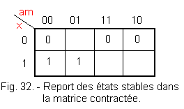
There are three boxes to fill in for transition states.
We will report the logical state of the output (1 or 0) for the steady state to which the transient state considered evolves.
The transient state 1 evolves towards the stable state ![]() for which L = 1
for which L = 1
The transient state 4 evolves towards the stable state ![]() for which L = 0
for which L = 0
The transient state 3 evolves towards the stable state ![]() for which L = 0
for which L = 0
Let's put these values in the matrix of Figure 32.
We get the Karnaugh chart from Figure 33.
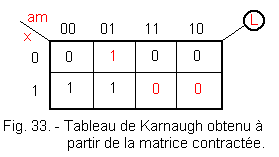
From this table of Karnaugh, the problem is again a combinatorial problem.
We can achieve the groupings as we have learned to do. They are represented in figure 34.

We obtain the following equation of L :
L = ![]() m
+
m
+ ![]() x
x
Let L = ![]() (m
+ x)
(m
+ x)
We find the equation obtained by the previous methods.
We have 2 methods to solve a sequential problem :
-
The generalized phase method
-
HUFFMAN's matrix method
We will prefer the Huffman method which is more abstract but more systematic and more secure. However, the generalized phase method has the advantage of allowing a visualization of the possible operating hazards and their eliminations easier. One can therefore only recommend the use of the phase method as verification of a scheme obtained by the method of Huffman to look for possible hazards.
Now let's look at Bistable Flip-Flops.
 Click here for the next lesson or in the summary provided for this purpose. Click here for the next lesson or in the summary provided for this purpose. |
|
 Previous Page Previous Page |
 Next Page Next Page |
Nombre de pages vues, à partir de cette date : le 27 Décembre 2019
Envoyez un courrier électronique à Administrateur Web Société pour toute question ou remarque concernant ce site Web.
Version du site : 10. 4. 12 - Site optimisation 1280 x 1024 pixels - Faculté de Nanterre - Dernière modification : 02 Septembre 2016.
Ce site Web a été Créé le, 14 Mars 1999 et ayant Rénové, en Septembre 2016.
